
It has been quite common to assume that market prices, and even the application of widely accepted “fair” asset valuation methods, are sufficient to comply with the arm’s length principle. However, this is not necessarily the case, as economic phenomena such as synergies have peculiar implications.
Synergies imply that the interaction of assets—often occurring when they are part of the same organization—generates a combined value greater than the sum of the value each asset would generate individually without interacting.
In terms of an asset transaction, this could mean that the value contribution to the acquiring entity is not necessarily equal to the amount lost by the selling entity.
Regarding the valuation of the asset in question, a widely accepted approach is the present value of discounted future cash flows. The primary challenge in this method is identifying the portion of a company’s profits attributable to the analyzed asset.
To simplify this issue, the Shapley value tool can help determine the profits that can be “fairly” attributed to a specific asset within a company.
The Shapley value is a wealth distribution method in cooperative game theory, assuming that all participants collaborate by forming a grand coalition. It is considered a “fair” distribution because it is the only one that satisfies certain desirable properties: efficiency, symmetry, linearity, and the null player property.
Given a group N (with n players) and a function υ : 2N → R with υ(∅) = 0, where ∅ denotes the empty set, the function v, which assigns subsets of real players, is called the characteristic function. The function v has the following meaning: if S is a coalition of players, then v(S)—the value of coalition S—describes the total sum of payments to the members of S that can be obtained through this cooperation.
According to the Shapley value, the amount that player i receives in a coalition game (v, N) is:
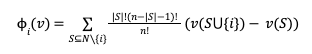
Where n is the total number of players, and the summation extends over all subsets of N that do not contain player i.
Example
Suppose we have three players {a, b, Δ}, where a represents the set of assets held by A (except Δ), and b represents the set of assets held by B, while Δ is an asset that is difficult to value.
Initially, the asset Δ is owned by A, and its potential sale to B is being analyzed. Thus, the estimation of the “fair” utility corresponding to asset Δ is:
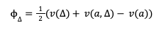
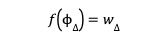
Where ∅ represents the annual utility of an asset, and w is the present value of the asset.
The price of asset Δ would then be:
Arm’s Length Implications
However, A should not be willing to sell asset Δ for a price lower than f(v(a,Δ) – v(a)), as otherwise, it would not compensate for the loss of utility that A incurs by ceasing to exploit asset Δ.
If the condition v(Δ) < v(a,Δ) – x(a) holds, meaning there is no restriction preventing this from happening, then w would not be arm’s length, despite being a “fair” price, as it would not be a price at which the asset owner would be willing to sell.
Additionally, if the condition v(a,Δ) – v(a) > v(b,Δ) – v(b) holds, the contract curve between A and B would be ∅. In other words, there would be no possible price at which the transaction could take place because, at any price, either A, B, or both would be worse off than before, thus violating the arm’s length principle.
The above analysis leads us to reflect that, while the primary objective of the transfer pricing framework is compliance with the arm’s length principle, a lack of information in the analysis may pose the risk of being unable to demonstrate or determine arm’s length prices. However, both market prices and theoretically “fair” prices can be acceptable alternatives, especially in the practical application of transfer pricing analysis.
JCG